Explanation By Example
Using USA LRFD combinations as an example| Base Combination | Expanded Combinations | |
|---|---|---|
| 1. 1.4D | 1.4D | 1 |
| 2. 1.2D + 1.6L + 0.5Lr | 1.2D + 1.6L + 0.5Lr 1.2D + 1.6L2 + 0.5Lr | 2 3 |
| 3. 1.2D + 1.6L + 0.5S | 1.2D + 1.6L + 0.5S 1.2D + 1.6L2 + 0.5S | 4 5 |
| 4. 1.2D + 1.6L + 0.5R | 1.2D + 1.6L + 0.5R 1.2D + 1.6L2 + 0.5R | 6 7 |
| 5. 1.2D + 1.6Lr + f1L | 1.2D + 1.6Lr + f1L 1.2D + 1.6Lr + f1L2 | 8 9 |
| 6. 1.2D + 1.6Lr + 0.5W,dn | 1.2D + 1.6Lr + 0.5W,dn 1.2D + 1.6Lr + 0.5W,dn2 | 10 11 |
| 7. 1.2D + 1.6S + f1L | 1.2D + 1.6S + f1L 1.2D + 1.6S + f1L2 | 12 13 |
| 8. 1.2D + 1.6S + 0.5W,dn | 1.2D + 1.6S + 0.5W,dn 1.2D + 1.6S + 0.5W,dn2 | 14 15 |
| 9. 1.2D + 1.6R + f1L | 1.2D + 1.6R + f1L 1.2D + 1.6R + f1L2 | 16 17 |
| 10. 1.2D + 1.6R + 0.5W,dn | 1.2D + 1.6R + 0.5W,dn 1.2D + 1.6R + 0.5W,dn2 | 18 19 |
| 11. 1.2D + 1.0W,dn + f1L + 0.5Lr | 1.2D + 1.0W,dn + f1L + 0.5Lr 1.2D + 1.0W,dn + f1L2 + 0.5Lr 1.2D + 1.0W,dn2 + f1L + 0.5Lr 1.2D + 1.0W,dn2 + f1L2 + 0.5Lr | 20 21 22 23 |
| 12. 1.2D + 1.0W,dn + f1L + 0.5S | 1.2D + 1.0W,dn + f1L + 0.5S 1.2D + 1.0W,dn + f1L2 + 0.5S 1.2D + 1.0W,dn2 + f1L + 0.5S 1.2D + 1.0W,dn2 + f1L2 + 0.5S | 24 25 26 27 |
| 13. 1.2D + 1.0W,dn + f1L + 0.5R | 1.2D + 1.0W,dn + f1L + 0.5R 1.2D + 1.0W,dn + f1L2 + 0.5R 1.2D + 1.0W,dn2 + f1L + 0.5R 1.2D + 1.0W,dn2 + f1L2 + 0.5R | 28 29 30 31 |
| 14. 1.2D + 1.0Ev + 1.0Eh + f1L + 0.2S | 1.2D + 1.0Ev + 1.0Eh + f1L + 0.2S 1.2D + 1.0Ev + 1.0Eh + f1L2 + 0.2S 1.2D + 1.0Ev + 1.0Eh2 + f1L + 0.2S 1.2D + 1.0Ev + 1.0Eh2 + f1L2 + 0.2S | 32 33 34 35 |
| 15. 0.9D + 1.0W,up | 0.9D + 1.0W,up 0.9D + 1.0W,up2 | 36 37 |
| 16. 0.9D - 1.0Ev + 1.0Eh | 0.9D - 1.0Ev + 1.0Eh 0.9D - 1.0Ev + 1.0Eh2 | 38 39 |
Key Points
- There are many more “expanded” load combinations than “base” load combinations
- You only INPUT the “base” load combinations into your “remote” widget. The solver automatically expands them out, based upon any alternate load types that you tell the solver exists.
- The solver internally calculates everything using the expanded combinations.
- Some solver OUTPUTS are base combinations, and some are expanded combinations. Be careful which is which!
Pay close attention to whether solver outputs are using base or expanded combinations, as this affects interpretation of results.
The Weird Stuff
Recombining Expanded into Base Combinations
Let’s take this combination as an example:| Base | Expanded |
|---|---|
| 0.9D + 1.0W,up | 0.9D + 1.0W,up 0.9D + 1.0W,up2 |
- W,up = “-0.9D”
- W,up2 = “0”
remote.LCTable.maxR(maximum reaction) will be equal to 0.9D (= 0.9D + 0)remote.LCTable.minRwill be equal to 0 (= 0.9D - 0.9D)- The signed absolutely maximum
remote.LCTable.Rwill be equal to 0.9D
Be very careful as to what result you’re actually looking for if you use these in your calculations!
Sorting of Expanded Load Combinations
In all of the outputs that include expanded load combinations, they are returned in the order that the solver has generated them in. That means that all the alternate load types are included in later indices. The first 16 load combinations look like the base combinations, but are actually the expanded combinations - NOT recombined!Visual Example
The diagrams show the envelope considering all different types of Q (Q1, Q2, Q3). Observe that Q1, Q2 and Q3 are not considered in the same load combination. The images below show that the bending demand is the same across different load types.


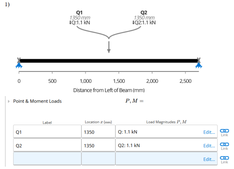
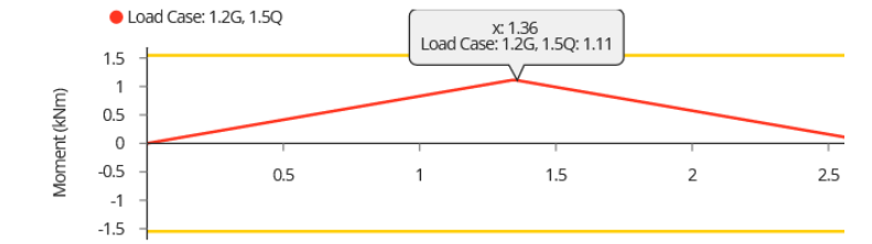
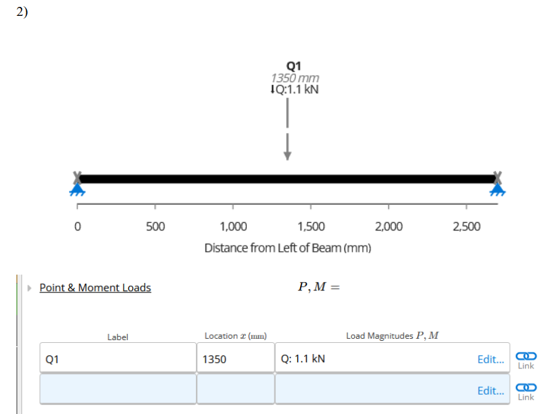
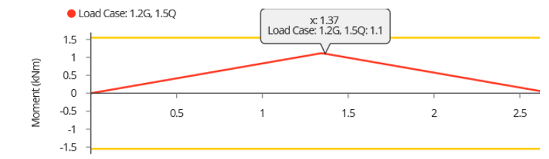
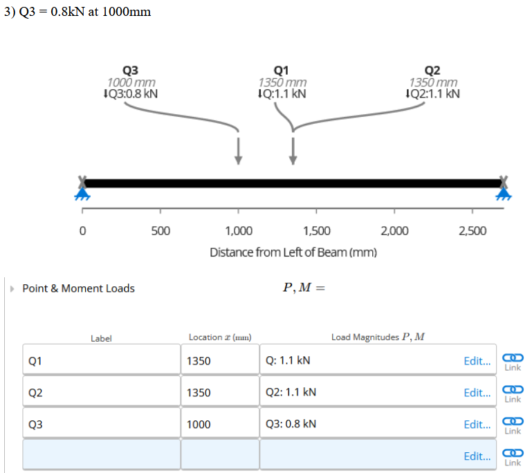
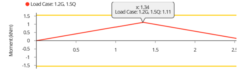
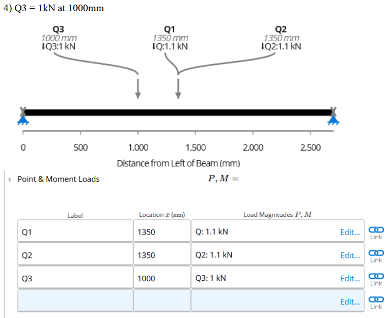
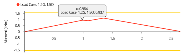
The envelope diagrams show the maximum effects from all non-concurrent load combinations, demonstrating how the solver handles multiple load types without combining them inappropriately.